Identifying performance bottlenecks in long-running processes often involves careful instrumentation ahead or guessing where the root of the problem may be. A very welcome set of tools are the ones that help you diagnose problems of live systems without modifying them. One important tool I recently came across is the pyflame profiler.
pyflame uses Linux’ ptrace(2) system call to take snapshots of the running
Python interpreter without the need for additional instrumentation. While it
introduces some overhead, it is much smaller than when using cProfile. The
most important aspect of pyflame is though that you can use it to profile
already running processes.
To install pyflame you can either follow the build instructions in its
documentation
or install it through conda: conda install -c conda-forge pyflame.
While writing this article, another Python profiler was published that is very
similar to pyflame: py-spy. A lot of the
content in this article is also helpful when working with py-spy; so
it’s worthwhile to keep reading even if you select this one. One of the reasons
py-spy exists is actually pyflame and its main limitation. As the
ptrace(2) system call is only available on Linux, pyflame is only available
on Linux. py-spy uses a slightly different approach and thus also runs on OSX
and Windows.
While pyflame is very handy when debugging an already running or
a long-running job, it’s not my only go-to profiler. In the case I have some
code where I know that something is slow, I normally setup a small script
with just the culprit. This script should use enough input data to highlight
any performance issues but should only use as much RAM and CPU that I can run
it very often on my laptop. To get a good understanding where the hotspot is,
I run this script using cProfile and then view the output in qcachegrind:
python -m cProfile -o output.cprofile script.py
pyprof2calltree -i output.cprofile -o output.cachegrind
Once I know which function is the main hotspot, I rerun my code several times
and record the timings of each line in the function that shall be tuned using
line_profiler. For this I use mostly
its IPython magic to do quick iterations with different inputs.
Looking at these timings I either dig one level deeper and optimize a lower
function or rethink the implementation of the current function to speed up
the code. This can either be improving the actual algorithm and its asymptotic
runtime complexity or a better implementation of the existing code using more
performant functions (e.g. vectorizing numerical code).
To illustrate the usage of pyflame, we use a small machine learning example. It is quite simple but already takes a significant amount of time to run:
from sklearn.ensemble import RandomForestRegressor

import pandas as pd


# Use New York Taxi trip data from january 2016 as medium size dataset
df = pd.read_csv(
    'yellow_tripdata_2016-01.csv',
    parse_dates=['tpep_pickup_datetime', 'tpep_dropoff_datetime'],
    infer_datetime_format=True
)
X = df[['extra', 'trip_distance', 'passenger_count', 'VendorID', 'payment_type']].values
y = df['total_amount']

estimator = RandomForestRegressor(n_estimators=20)
estimator.fit(X, y)
We execute this code using pyflame -x -o profile.txt -t python scikit-example.py.
The output of pyflame is then rendered using
flamegraph.pl <profile.txt >profile.svg using Brendan Gregg’s FlameGraph
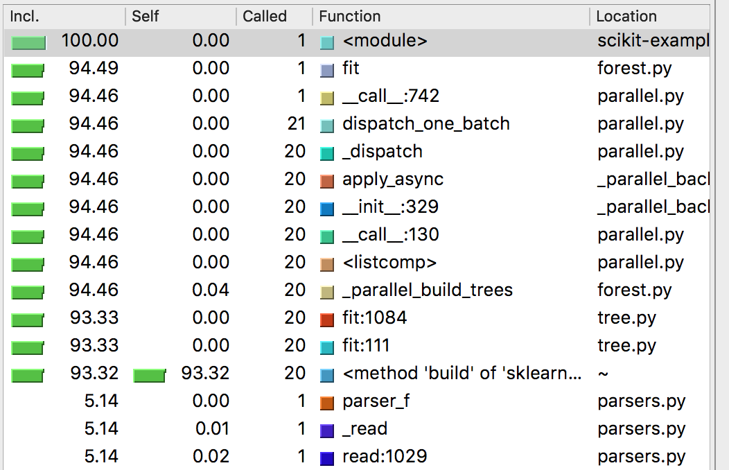
script. This results in the below
pictured flamegraph. We have used the -x flag here to hide “idle” time. This
is not actually time where the process is idling but time where pyflame cannot
observe the stacktrace. In this case, you should also produce a C++ flamegraph
as mentioned later in the article.

The birds-eye view already shows us already the three parts of the program: The loading of the data with the CSV parser as the widest section, then the fitting of the model which takes a significant amount of time and finally the prediction step. While the prediction is quite fast, it is still noticeable in the flamegraph as it has a much deeper stack as all the other parts. The output of the flamegraph.pl script is an interactive SVG. This means that you can click on any part of the stack and the tool zooms into the selection.
The main driver for me to use pyflame is when I want to get an overview of
a large program. Often, we are simply aware that we have a performance issue
but can only guess in which part of the program. Sometimes this even happens
only in a productive setup. Then we can simply attach to the already running
process and profile it for a certain time frame and have a look at the
flamegraph afterwards.
As pyflame has a very small overhead, we can attach it to real production
processes. Especially the overhead is acceptable when you’re in an incident
situation due to yet unresolved performance issues. But you need to be aware
that profiling still introduces some overhead on your general system. Thus you
need to be aware that the system will still run slower when it’s monitored.
Just not as slow as if you would have used cProfile.
In addition to the ability to attach to running processes, an important aspect
for me in pyflame is that it directly generates flamegraphs. For a quick
overview of a programs performance hotspots, flamegraphs are my favorite
visualization technique in any programming language I use. Their advantage is
that you can see on a single screen where potential performance bottlenecks
are; independent on how deep they are in the stack. Especially when you use
the FlameGraph scripts from Brendan Gregg
to generate these visualizations, you can then also dig deeper into the
stacktraces to only view the interesting parts.
A flamegraph itself is a visualization of several accumulated stackframes.
These frames are visualized from bottom to top, i.e. the most outer function
(mostly main) will be at the bottom of the visualization. The frames are
then sorted alphabetically from top to bottom. This means that stackframes
that have a common origin also appear next to each other. Thus this shows
in which parts of the call stack we spend most of the time. These are the
hotspots one is looking for when diagnosing a performance problem in a running
process.
This kind of visualization shows us the hotspots of the program. Due to its alphabetical ordering of the strackframes, it shows where most of the time is spent but not when. To get the time information, one can sort the stackframes chronologically, not alphabetically. This alteration is then called a flamechart and is for example used in Chrome’s JS profiler.
While a Python programmer is mostly interested in the Python view of a program,
it often happens that we spend a long time in a Python function that calls
native code. To profile native code on Linux, one can use perf and dtrace
on OSX. Both will produce a flamegraph using the following commands. Sadly,
they will only show the names of the C functions in the Python interpreter,
not the actual Python stacktraces. In the case of scientific Python code,
this is very often still informative.
To generate a native CPU flamegraph of the above scikit-learn example, you will
need to record the events with perf first:
perf record -F 999 -g -- python scikit-example.py. Afterwards you can pass
the output of perf through some pre-processing scripts to the flamegraph.pl
script to get an SVG similar to the the one generated before using pyflame:
perf record -F 999 -g -- python scikit-example.py
perf script | ./FlameGraph/stackcollapse-perf.pl | ./FlameGraph/flamegraph.pl > profile-perf.svg
In the case of the scikit-learn example, this is an important step to do.
One of the limitations of pyflame is that it only shows the stacktraces while
the GIL is held. In the case of the scikit-learn model used, a lot of work is
done without holding Python’s GIL. Thus the native stacktrace shows a different
ratio between fit and loading data. The time without a GIL is normally shown as
IDLE in pyflame’s output. As we have used the -x flag on the profile run,
this was omitted automatically from our previous FlameGraph.
pyflame and perf are both only available on Linux but when you’re on OSX and
still want to generate CPU flamegraphs for native code, you can use dtrace.
Also, as mentioned in the introduction, there is a new project called py-spy
that should give you similar functionality to pyflame but also on OSX.
sudo dtrace -c 'python scikit-example.py' -o out.stacks -n 'profile-997 /pid == $target/{ @[ustack(100)] = count(); }'
./stackcollapse.pl out.stacks | ./flamegraph.pl > profile.svgWhen we either want to profile an already running Python process or get a comprehensive overview of the CPU hotspots, we can utilize pyflame to get a profile. As pyflame is a statistical profiler, it adds no significant runtime overhead to the actual program and does not either need any kind of instrumentation. With the flamegraph representation of the result, we can see at a glance what the most expensive code sections of a program are, independently of when they were invoked.